Fifty ways to leave your model

The problem is all inside your head, she said to me.
The answer is easy if you take it logically.
I’d like to help you in your struggle to be free.
There must be fifty^2.2162 ways to leave your lovermodel.

Suppose we have a theory about the mechanism that sustains insomnia. The theory can be roughly summarized in a (dynamic) causal graph model like so:

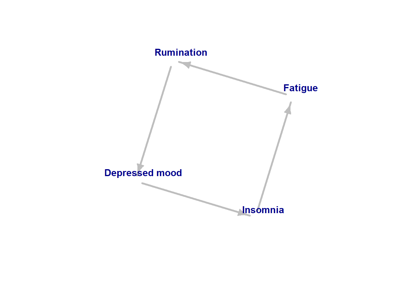
Figure 1: Example causal model.

Suppose our model is supported by reliable observational data which suggests that the four concepts in the model above comprise a necessary and sufficient set of components to describe insomnia maintenance. However, the observational data are purely qualitative, and cannot tell us anything about the causal relationships between these concepts. We nonetheless draw in some arrows (perhaps based on our clinical or scientific intuition) and get the model above. Given no data to support our causal beliefs, how likely are we to have drawn the right model by chance? How many alternative models could we have considered for these variables?

Generating alternative causal models can be expressed as a combinatorial problem. There are a number variable pairs that we can have a causal hypothesis about (e.g. “A, B”), and for each pair of variables there is a finite set of possible causal relationships (edges) that we could hypothesize e.g. (“→”, “←”). In other words there are ||edges|| hypotheses to choose from (double vertical lines stand for the number of elements, or cardinality, of the set of edges), and we are going to choose an edge pairs number of times (with replacement). Using the rule of product, assuming all edges are possible for all pairs, we can calculate the number of possible models like so:

\[ \begin{equation} Models=||edges||^{pairs} \tag{1} \end{equation} \]

How many edges are there? An undirected graph has only 2 possible edges for every pair of nodes (“A ー B” and “A ⊥ B”). A directed acyclic graph has three possible edges (“A → B”, “A ← B”, “A ⊥ B”), and a dynamic causal model has four (“A → B”, “A ← B”, “A ⊥ B”, and “A ↔︎ B”). Since our example model is dynamic (it contains a feedback loop), we must allow for dynamic “↔︎” edges. Then we have four possible edges in the set of edges:

\[ \begin{equation} ||edges||=4 \tag{2} \end{equation} \] How many node pairs are there? For two nodes (A,B) there is only one pair we can make (AB, which is equivalent to BA), and for three nodes (A,B,C) there are only three pairs we can make (AB, AC, BC). Since the number of pairs grows exponentially with the number of nodes, it becomes cumbersome to count out the possible pairs after a while. However, if we know the number of nodes we can derive the number of pairs automatically.

One way to count the number of pairs would be to draw a graph of our nodes with an edge between every pair of nodes, and then count the number of edges. Since every pair of nodes have an edge between them, the number of edges equals the number of pairs. Below is such a graph for our example model. There are 6 edges in this graph, which is also the number of possible pairs of variables (AB, AC, AD, BC, BD, CD).

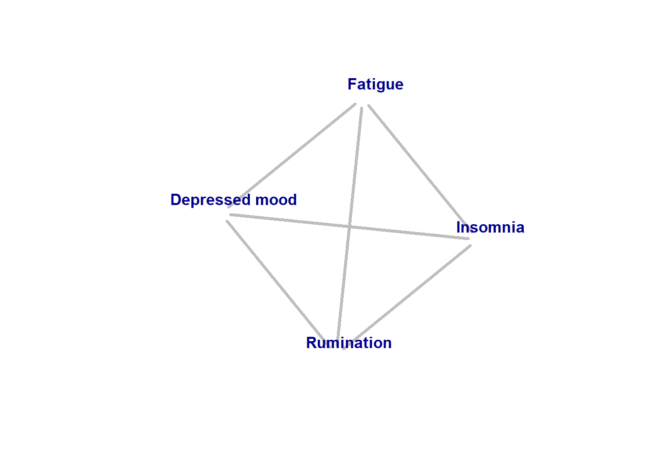
Figure 2: All possible pairs in example model, represented as undirected edges.

A graph where all pairs are connected is called a fully connected graph. In a fully connected graph, we also know the number of other nodes each node is connected to; the vertex number V of each node. Since all nodes are connected to all other nodes, each node has a vertex number of n-1 (all nodes, minus the one we’re looking at). Since all nodes have the same vertex number, we can multiply n-1 by the number of nodes n to get the total vertex number V_total of the graph.

Now, if we know the number of nodes and the total vertex number V_total of a graph, we can use this information to derive the number of edges (i.e. the number of variable pairs). The equation looks like this:

\[ \begin{equation} pairs=\frac{V_{total}}{2} \tag{3} \end{equation} \]

In our example model (figure 1), we have four nodes. Therefore:

\[ \begin{equation} pairs=\frac{V_{total}}{2}=\frac{nodes(nodes-1)}{2}=\frac{4(4-1)}{2}=6 \tag{4} \end{equation} \] Now that we know both the number of possible causal relationships (edge types) and the number of possible variables pairs (edges) in our example model, we can plug them into equation 1 to find the total number of alternative models:

\[ \begin{equation} Models=||edges||^{pairs}=4^6=4096 \tag{5} \end{equation} \]

Yikes. Even with only four variables, we have 4096¹ possible causal models to choose from! If we add another variable to the model, the number of alternatives grows to over a million. In other words, in absence of any data we should probably not take our model too seriously.

What could we use this information for? First of all, it clearly indicates we ought to take causal hypotheses about complex systems (like symptom networks) with a hefty grain of salt before we have data on the table. For a system of only 4 variables, you have about a 0.024% chance of getting the causal structure right on the first try.

Second, it might be interesting to use information about equivalent models to evaluate the falsifying power of different study outcomes. In the context of causal models, severe empirical studies help us rule out/falsify certain causal hypotheses. This means that, given data, some variable pairs have fewer edges to choose from, because some edges are now ruled out by the data. In order to calculate how many models are ruled out by a certain study outcome, we need to modify formula 1 somewhat. For models with pairs number of pairs, with a different number of possible edges for each pair i, we can calculate the number of possible models like so²:

\[ \begin{equation} Models=\displaystyle\prod_{i=1}^{pairs} edges_{i} \tag{6} \end{equation} \] Suppose we conduct an experiment which shows that insomnia causes fatigue and not the other way around (with absolute certainty, for the sake of illustration). Thus, we have determined (Insomnia → Fatigue) and falsified (Insomnia ← Fatigue), (Insomnia ↔︎ Fatigue) and (Insomnia ⊥ Fatigue). Now we have 5 pairs with 4 possible edges, and 1 pair (insomnia, fatigue) with only 1 possible edge (“→”). We can find the number of models that are equivalent with our finding like so:

\[ \begin{equation} Models=\displaystyle\prod_{i=1}^{pairs} edges_{i}=4\times4\times4\times4\times4\times1=4^51^1=1024 \tag{7} \end{equation} \] Perhaps we could use this information to assess the theoretical value of conducting particular studies. For example, if we are considering whether to conduct an experiment that would give us near certain knowledge about a particular edge in our causal graph, that experiment would exclude 1-1024/4096=75% of all possible causal theories we could make about these variables. Compare this to an observational study that would be able to rule out one edge from each of three pairs:

\[ \begin{equation} Models=\displaystyle\prod_{i=1}^{pairs} edges_{i}=4\times4\times4\times3\times3\times3=4^33^3=1728 \tag{8} \end{equation} \]

Thus, even though the observational study rules out as many edges overall as our experiment, it only rules out about ¾ as many models as the experiment does. In other words, if our goal is simply to rule out/falsify as many causal models as possible, the experiment would be the more efficient study choice in this case. To the extent that we can say something about the falsifying power of different study designs before they are conducted, the reduction in alternative models post data could be used to decide which study would be the most efficient to conduct next.