Quantifying the corroboration of a finding
By Peder M. Isager
April 12, 2019
Abstract
In a fourthcoming paper by members of the Open Science Collaboration, we outline how one could use quantitative estimates of “replication value” to guide study selection in replication research. We define replication value conceptually as a ratio of “impact” over “corroboration,” and we show how to derive quantifiable estimates from this definition. Here I will try to identify a reasonable and quantitative operationalization of corroboration. I first propose to approximate corroboration through the more narrow concept “precision of the estimate” (figure 1). I then quantify precision of the estimate as the variance of Fisher’s Z, which only depends on sample size (although the variance of the common language effect size A could also be used for group comparisons, if information about group sample sizes is available. See table 1 for a summary).
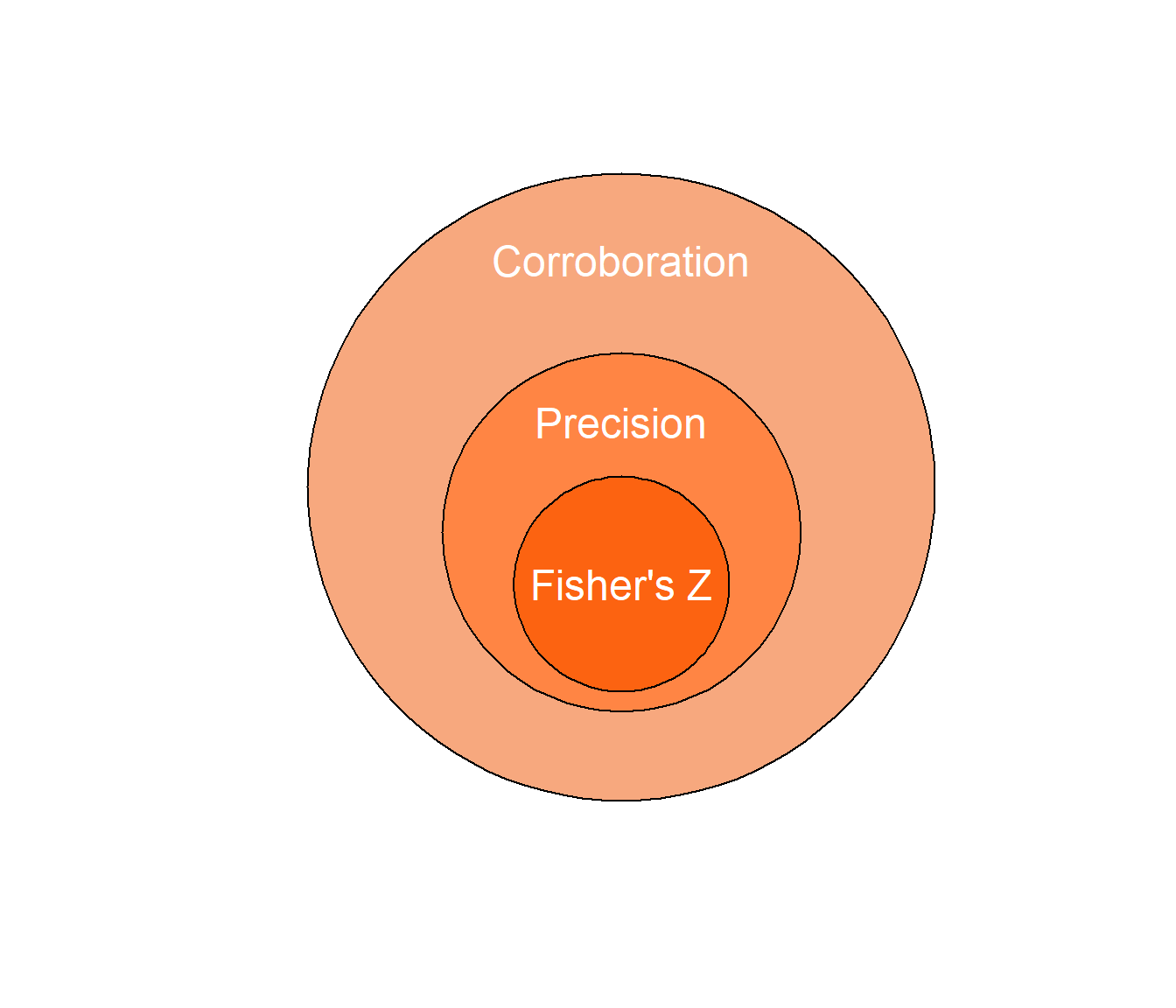
Figure 1: Illustration of the nested conceptual relationship between corroboration, precision and the Fisher’s Z statistic.
Needles in haystacks
When we seek to replicate findings in psychology, we may often face the problem that there are multiple findings we could replicate, but we only have resources available to address one or a few of our options. This means that we will have to decide which finding would be the most valuable to spend our time replicating. But the process of study selection can itself be a challenge. For example, in a replication effort I am currently involved with, we have more than 1000 studies we could consider for replication, each of which will contain multiple findings. We would like to discover and choose from the most valuable findings to replicate in this sample, but we simply do not have the time or cognitive capacity available to manually inspect and compare 1000 studies to each other. Is there a way to evaluate this set of studies and identify the most promising replication candidates, without committing years of time to combing through all the individual studies?
Quantifying replication value
Together with members of the Open Science collaboration I am currently trying to develop an approach for quantifying the “replication value” of published findings through formulas. If we could quantify estimates of replication, and if we could make sure that these estimates could be calculated relatively quickly, then this should allow researchers to evaluate large sets of findings and identify promising replication candidates. Manual inspection will still be required, but can be focused on the most promising candidates from the formula evaluation. As such, the aim is to increase the efficiency of manual inspection efforts, and to maximize the chance that high-value replication targets are discovered. We propose that the replication value of a finding can be thought of as a combination of the impact and the corroboration of that finding in the literature:
\[\begin{equation} RV=\frac{Impact}{Corroboration} \tag{1} \end{equation}\]
In words, the more impactful a study has become, the higher its replication value (“RV” in formula) will be. Conversely, the better corroborated a finding has become, the lower its replication value will be. We can gain an understanding of what researchers might take as indicators of “impact” and “corroboration” by surveying the literature of published replication studies. In a previous blog post I provide a brief summary of the most common factors that researchers seem to take into account.
There are multiple issues and caveats that will need to be considered when trying to approximate the “true” replication value of a finding through quantitative information. Among other things, we need to know whether formula 1 captures our conceptual understanding of replication value, whether it can be expressed in quantitative terms, and if so, how to operationalize the concepts contained in formula 1 numerically. In this post I will deal with one rather fundamental question: How do we quantify corroboration?
Quantifying corroboration
By “corroboration,” I generally mean something akin to the definition held by the Lakatosian falsificationist (e.g. Hands 2008; Lakatos 1978). That is, a prediction (or finding) of the form “X is Y” achieves corroboration if we fail to falsify it after subjecting the prediction to a severe test1. Further, generating this kind of corroboration is a hallmark of scientific progress, even if we accept that all theories are born false (Hands 2008). There are many aspects of corroboration that a researcher could care about, which subsequently informs the quantitative information they would be interested in (Lakens 2019). For example, we might want to prioritize findings for replication that have low evidence in favor of certain hypotheses compared to others (Field et al. 2018). Or we may want to prioritize findings that display signs of biased and/or erroneous reporting (Brown and Heathers 2017; Heathers et al. 2018; Simonsohn, Nelson, and Simmons 2014; Dwan et al. 2008; Nuijten et al. 2017; Kerr 1998). Or perhaps we simply want to replicate findings where we are surprised about the likelihood of the data under the null hypothesis. Focusing on different aspects of corroboration would lead to different justifications for any quantifiable operationalization of corroboration. Here we choose to focus on precision, and the following discussion of operationalizations is based on the assumption that our predictions are corroborated by precise estimates of parameters. The arguments that follow will not necessarily hold when focusing on other aspects of corroboration (e.g. Field et al. 2018).
Precision of the estimate can normally be thought of as the variance, standard error, or confidence/credible interval of a measurement (Borenstein, chapter 8). However, precision can also be related to qualitative estimates (e.g. people generally experience set S of side effects after taking drug D) and predictions involving multiple estimates (e.g. people experience side effect X, Y, and Z, with magnitude A, B and C, respectively, after taking drug D). More generally, precision can be thought of as the reciprocal to uncertainty. That is, for any estimand (a set, a magnitude, a mean, etc.), the less uncertain we are about whether it could be this way or that, the more precisely it is estimated. Precision can be considered one subcategory of what determines the corroboration of a finding. Everything else being equal, we may assume that a finding that has been estimated precisely has attained more corroboration than a finding that has been estimated imprecisely. Consequently, we may also assume that, everything else being equal, a precisely measured estimate is less replication-worthy than an imprecisely measured estimate, which is what follows from our conceptual definition of replication value in formula 1.
Of course, everything else is usually not equal, and corroboration as a construct encompasses much more than the precision of an estimate (figure 1). This is partly why manual inspection should always be part of evaluating whether one finding is truly more worth replicating than another. Still, we consider it plausible that precision of the estimate is positively correlated with corroboration on average. By substituting precision for corroboration in the replication value formula 1, we will essentially prioritize findings for replication that have been imprecisely measured in the literature thus far.
When comparing the precision of a set of estimates, we may want to compare two or more effects that stem from different designs, and that are expressed on different scales. That is, sometimes we may wish to compare effects expressed in Cohen’s d to effects expressed in Pearson’s r, odds ratio, etc. In order to compare effects expressed on different scales, we need an estimate of precision that is comparable across the scales. Otherwise, we cannot meaningfully compare the corroboration of two different kinds of effects. Consider a confidence interval CI[2.27, 14.04] for an effect expressed in units of Cohen’s d. In the context of most behavioral research, this would be considered a highly imprecise measurement. Now consider a confidence interval CI[0.75, 0.99] expressed in units of Pearson’s r. If directly compared, the latter interval might appear more precise than the former, but this is simply due to the fact that Pearson’s r is a non-linear scale bounded between -1 and 1, whereas Cohen’s d is a linear scale bounded between -∞ and ∞. In fact, the two intervals in this example are the same interval, expressed in two units of measurement. We can compare their precision only if we first convert either interval into the scale of the other, or convert both intervals into some other common unit of measurement. It is not meaningful to compare intervals measured on different scales directly.
This problem is similar to that faced by meta-analysts who want to compare effect sizes measured on different scales (Borenstein 2009, chap. 7). However, the two problems are not quite the same. For example, meta-analyses ideally deal with studies on the same effect that are either “close” replications (LeBel et al. 2018), or at least conceptually similar. The replication value, on the other hand, should be comparable even for studies that are not on the same topic. In addition, the effect size is often the statistic of interest in traditional meta-analysis. In contrast, since the size of the effect is orthogonal to the precision of the estimate of the effect, effect size should be irrelevant for our corroboration estimate.
Requirements for a precision statistic
In order for a precision statistic to be useful in the context of the replication value, we should expect it to adhere to the following requirements:
Standardization: The measure must express precision on a standardized scale. If calculated for a number of estimates, the precision of the estimates must always be placed on the same scale.
Meta-analytic updating: we must be able to update the precision statistic after a replication is performed. Replication generally adds information about a finding, and should tend to increase the precision of an estimate and thus decrease the replication value of a finding.
Size independence: The measure must not depend on the size of the effect.
Exhaustiveness: The measure must accurately represent the precision of the estimate. Therefore, the measure should take all relevant aspects of the precision into account when they are available, such as the standard deviation of the estimate, the sample size, the between-condition correlation for repeated measures, etc.
Each requirement is supported by a specific rationale related to the desired functions of the replication value. If the standardization requirement is violated, it becomes impossible to know if differences between effects are due to differences in impact and precision, or if the compared effects are equally precise but measured on different scales. If the meta-analytic updating requirement is violated, there is no mechanism for updating the precision estimate after replications are conducted. This would disrupt a central feature of the replication value; after a finding is replicated, its replication value should decrease. If the effect-size independence requirement is violated, the replication value will become biased (either favorably or unfavorably) towards findings with a large effect size. This is undesirable if we assume that the goal of replication is to reduce uncertainty in an estimate regardless of whether the true effect is large, small or zero (we may not always want to assume this of course). If the exhaustiveness requirement is violated, we risk misrepresenting the actual precision of certain measures. For example, two estimates may have the same sample size and yet, if standard deviations or within-subject correlation differs substantially between the estimates, one estimate can be much more precise than the other. The exhaustiveness requirement could be considered less critical than the other three however. As long as the error introduced by violating it is random, the precision estimate becomes less accurate by not accounting for all relevant factors, but not categorically invalid. It still tracks our conceptual understanding of “precision” to some degree. However, more serious issues arise when not accounting for relevant information leads to systematic bias. For example, if we ignore inter-trial correlation and the fact that each subject contributes at least two data points in within-subject designs, the precision of the estimate (and hence, the replication value) of within-subject measurements will be overestimated compared to between-subjects measurements. In this case, not accounting for the difference in design would ultimately lead us to violate the standardization requirement.
Candidate statistics
There are several potential candidate statistics we could consider as an operationalization of precision, each of which will have benefits and limitations (see table 1 for summary). I will here deal with several of them in turn, show the benefits and limitations of each approach, and give a general justification for the statistic that appears in the example replication value formula we provide in our forthcoming manuscript.
P-values
P-values are related to precision in that they tend to become smaller with increasing precision of the estimate, provided that the null hypothesis is false. P-values also have the desirable feature that they are very often reported, which would make the calculation of the replication value feasible for the large majority of effects in the published literature. However, p-values from null-hypothesis significance tests (NHST) violate the size independence requirement. That is, p-values behave differently when the true effect is zero compared to when the true effect is not zero. Because p-values are always uniformly distributed under the null, they never change systematically with increases in measurement precision of a true null effect. In practice, this means that it will not be possible to lower the p-value of a true null effect by replicating it, which violates the requirement of meta-analytic updating. In addition, when there is a true effect, p-values entail different precision estimates depending on the size of the effect. That is, as the size of the true effect grows large, even very imprecisely measured effects will tend to yield data that is extremely unlikely given that the null hypothesis is true (i.e. small p-values). Of course, there might be other aspects of corroboration besides precision for which p-values would be a suitable operationalization.
Bayes Factors
Bayes factors are related to evidence for the null and alternative hypothesis, and - unlike p-values under NHST - do quantify relative support for the null-hypothesis (relative to a specified alternative hypothesis). Bayes factors require the specification of a prior, which is dependent on the research question and can differ between researchers. This threatens violation of the standardization requirement. Bayes factors also violate the size independence requirement. That is, a large but imprecisely measured effect can yield the same amount of Bayesian evidence as a small but precisely measured effect if we change the hypotheses being compared. Keep in mind that this is only problematic given that the overarching goal is to approximate the broad concept of “corroboration” through the more narrow concept of “precision.” One could easily make case that Bayesian “evidence” is another valid way of approximating corroboration, and a general framework for study selection in replication research that builds on Bayes factors has been outlined in detail elsewhere (Field et al. 2018).
Variance2 of the estimate
The variance is perhaps the most direct measure of estimate precision. Unlike p-values and Bayes factors, the variance clearly respects the size independence requirement. I.e. it tends to become smaller with increasingly precise estimates, regardless of the effect size of the estimate. However, the variance of raw estimates would still violate the standardization requirement as soon as we compare estimates that are measured on different scales. We can solve this issue by converting all effects into the same standardized scale and then calculating the variance of the standardized effects. There are several scales we could use (Cohen’s d, Pearson’s r, Fisher’s Z, etc.) so we consider the variance formulas for all of them in turn. All variance estimates considered here satisfy the standardization requirement.
Variance of Cohen’s d / Hedge’s g
The variance of Cohen’s d (for independent groups) is defined as (Borenstein 2009, formula 4.20):
\[ \begin{equation} V_d=\frac{n_1+n_2}{n_1n_2}+\frac{d^2}{2(n_1+n_2)} \tag{2} \end{equation} \]
where n is the group sample size, and d is the effect size Cohen’s d for independent groups. Notice the use of d2 in the right hand side of the expression. This leads the variance of d to increase with the effect size d. This means that the variance of d is, at least to some extent, dependent on the effect size d, and thus it is in violation of the size independence requirement.
The variance of Hedge’s g is simply the variance of d multiplied by a correction factor J (Borenstein 2009, formula 4.22 & 4.24). Hedge’s g therefore depends on the effect size d as well, and is in violation of the size independence requirement.
\[ \begin{equation} J=1-\frac{3}{4df-1} \tag{3} \end{equation} \]
The variance of Cohen’s dz (for repeated measures/matched groups/pre-post test scores) is defined as (Borenstein 2009, formula 4.28):
\[ \begin{equation} V_{d_z}=(\frac{1}{n}+\frac{d_z^2}{2n})2(1-r) \tag{4} \end{equation} \]
where n is the number of pairs, dz is the effect size Cohen’s d for dependent groups, and r is the correlation between pairs of observations. Notice that, as with Cohen’s d for independent groups, dz2 appears in the right hand side of this expression, meaning that the variance of dz will be dependent on the effect size dz.
Variance of Pearson’s r
The variance of Pearson’s r is defined as (Borenstein 2009, formula 6.1):
\[ \begin{equation} V_r=\frac{(1-r^2)^2}{n-1} \tag{5} \end{equation} \]
Again, notice the use of r2 in the right side of the expression. In this case, since r2 is subtracted from the numerator, Vr will tend to become smaller as r becomes larger. The variance of r thus depends on the effect size r, and is therefore in violation of the size independence requirement.
Because the variance of r depends heavily on the strength of the correlation, it is more common to convert the correlation to Fisher’s Z scale, and later calculate the variance estimates of Fisher’s Z back to values of r (Borenstein 2009, equation 6.2, 6.3, and 6.5). However, because Pearson’s r is bounded between 0 and 1, this method produces non-normally distributed intervals around r that still depend on the strength of the correlation, such that stronger correlations will tend to have smaller variances.
Variance of log odds ratio
The variance of the log odds ratio is given by (Borenstein 2009, formula 5.10):
\[ \begin{equation} V_{LogOddsRatio}=\frac{1}{A}+\frac{1}{B}+\frac{1}{C}+\frac{1}{D} \tag{6} \end{equation} \]
where A, B, C and D are the four events involved (Borenstein 2009, table 5.1). Though perhaps less intuitive than for d and r, the variance of the log odds ratio is also dependent on the size of the effect. This is due to the fact that for any two odds, the variance of the odds ratio becomes larger the more extreme both of the individual odds are. On the one hand, both odds could be extreme in the same direction, which would give a large variance for the log odds ratio, but a small log odds ratio. On the other hand, if the log odds ratio is large, at least one of the individual odds involved must be large. In other words, the variance will tend to become larger with larger log odds ratios, which means the variance depends on the size of the odds involved. Ultimately, this variance formula is also in violation of the size independence requirement.
Variance of Fisher’s Z
The variance of Fisher’s Z is defined as (Borenstein 2009, formula 6.3):
\[ \begin{equation} V_Z=\frac{1}{n-3} \tag{7} \end{equation} \] where n is the sample size. Unlike the previous variance measurements, the variance of Z is not in violation of the size independence requirement. That is, there is no relationship between the Fisher Z effect size and the variance estimate VZ for that effect.
However, the formula for VZ is in violation of the exhaustiveness requirement. In order to appreciate this, suppose we convert a Cohen’s d effect size estimate for independent groups (Borenstein 2009, formula 4.18) to Fisher’s Z. If we calculate the variance for the effect measured in Cohen’s d, we will take into consideration both total sample size, the relative sample size of the compared groups, and the standard deviation of the estimate, because these factors are all contained within the formula for the variance of d. However, when we convert Cohen’s d into Fisher’s Z, we must also re-calculate the variance, now using the formula for VZ. Because VZ only depends on the sample size, we effectively lose the extra information that was contained within Vd during conversion from d to Z.
Variance of A (nonparametric “common language effect size”)
The common language effect size (CLES. Ruscio 2008; Grissom and Kim 2001) is a standardized measure of the parameter Pr(Y1>Y2), or the probability that a randomly chosen member of group 1 scores higher than a randomly chosen member of group 2. The non-parametric version of this effect size (denoted A) is robust to violation of certain parametric assumptions that are frequently violated in practice, such as normality and heterogeneity of variances. When comparing effects where these parametric assumptions are likely to be violated, A is arguably the most appropriate scale on which to standardize effects.
Variance of A is defined as (Ruscio 2008, formula 9):
\[ \begin{equation} V_A=[(1/n_1)+(1/n_2)+(1/n_1n_2)]/12 \tag{8} \end{equation} \]
where n1 and n2 are the group sample sizes. This variance estimate is very similar to VZ, except that is also takes the group base rates into account (for a given n1+n2, n1*n2 is largest when n1=n2). Like VZ, VA is not in violation of the size independence requirement, but it is in violation of the exhaustiveness requirement. VA ignores some information about precision, such as the standard deviation of the estimate, even in cases where that information is available and relevant.
Discussion regarding the use of variance
In summary, surveying the available formulas for standardized variance estimates reveals some flaws with all of them, given the requirements imposed by our definition of precision. However, some are more problematic than others. Vd, Vg, Vr, and VLogOddsRatio all violate the size independence requirement. Unless we explicitly want to bias the replication value based on the size of effects, none of these variance estimates are recommended for use in a replication value formula.
VZ and VA are more promising alternatives. They both adhere to all requirements except exhaustiveness. However, there may be no way to avoid some loss of information if the goal is to compare measures on different effect size scales. We have to standardize all estimates to the same scale to make comparisons, and information unique to each effect size scale will be lost during this standardization process. Violation of the exhaustiveness requirement may be tolerable, given that sample size normally is the major determinant of estimate precision, even in equations that take more information into account (Borenstein 2009, chap. 8). I.e. we may accept the loss of information about group variances, group base rates, etc., if we can assume that for the large majority of cases, these factors only play a lesser role in determining estimate precision relative to sample size.
VA may be slightly more informative than VZ because it takes the ratio of the group sizes into account. However, VZ is a more widely applicable formula because VA can only be calculated for cases where there are two groups to compare. For this reason, we choose VZ as our operationalization of precision for examples discussed in our forthcoming manuscript. However, note that for sets of findings that only include comparisons between two groups, VA might be a more accurate measure.
There are a few pragmatic benefits to using VZ as a measure of precision, beyond it’s adherence to most of the requirements above. First, the sample size is often reported directly in manuscripts, and may even be possible to extract automatically in many cases (e.g. using Statcheck to extract degrees of freedom, Nuijten et al. 2017), which means that the replication value can be calculated for most reported effects with minimal effort. Second, VZ can be used more flexibly than other variance measures, because it is not dependent on knowing the effect size of a particular estimate. This has some practical benefits. For example, if a researcher needs to evaluate the replication value of 100 studies, and it is not feasible to identify the theoretically critical result in all of the studies, the researcher could calculate VZ using the total sample size in each individual study as a rough first guide to the replication value of individual the findings reported within.
However, by calculating VZ from pure sample sizes, we will introduce a more serious violation of the exhaustiveness requirement by ignoring the statistical design of the studies we intend to compare, which is another major determinant of precision (Borenstein 2009, chap. 8). As one example, a paired samples t-test has better precision for the difference score that is calculated between the two measurements than an independent samples t-test, partly because the participants contribute twice as many data points in the paired design, and partly because of within-subject correlation (see Lakens 2016 for a detailed explanation). Another example is the differences in precision when estimating a main effect vs an interaction effect using the same sample size (see Simonsohn 2015 for a discussion). We can attempt to mitigate these issues, however, by converting the sample sizes from within-subject and interaction designs into the corresponding sample size that would achieve the same precision for a main effect in a between-subjects design. This way, samples sizes from different designs can be reasonably compared on the same scale of precision. At present I am only able to provide a method for conversion between a within-subjects design and a between-subjects design. In the future, however, I hope to be able to provide a similar method for conversion between an interaction effect and a main effect as well, based on the derivations provided by Simonsohn (2015).
Converting within-subjects sample size into between-subjects sample size
Following equation 47 in Maxwell and Delaney (2004, chap. 11), if we assume normal distributions and compound symmetry, and if we ignore the difference in degrees of freedom between the two types of tests, we can solve for NB and convert the sample size of a within-subject sample into an estimate of a corresponding between-subject sample:
\[ \begin{equation} N_B=\frac{N_Wa}{1-ρ} \tag{9} \end{equation} \]
where NW is the sample size of the within-subject design, ρ is the within-subject correlation, a is the number of groups that each subject contributes data points to, and NB is the estimated sample size that a between-subject study would need to reach the same level of precision.
The population parameter ρ is usually estimated from the within-subject correlation r in the sample. A practical issue is that this value is very rarely reported in published manuscripts. In these cases, it is possible to calculate r from summary statistics. For example, if we has access to the t-value, Cohen’s daverage (Borenstein 2009, equation 4.18), and the sample size NW, we can calculate r by solving for r in Dunlap et al. (1996, equation 3):
\[ \begin{equation} r=\frac{2t^2-d_{average}^2N_W}{2t^2} \tag{10} \end{equation} \]
Or, if we has access to the standard error of the difference and the standard error of both groups, we could calculate r by solving for r in Lakens (2013, formula 8):
\[ \begin{equation} r=\frac{SD_1^2+SD_2^2-S_{diff}^2}{2SD_1SD_2} \tag{11} \end{equation} \]
If we does not have access to these summary statistics or the raw data, we could estimate ρ based on r in conceptually similar studies. If there are no realistic reference points for ρ whatsoever, we could potentially consider setting ρ to 0. NW will still receive a correction in this case from being multiplied by a. Note however, that this is a very conservative assumption, and unlikely to be realistic in most cases. Moreover, the choice of 0 over any other arbitrary value of ρ is motivated by nothing but a desire to be conservative.
Limitations when ignoring details of the study design
In certain situations, it might not be feasible or even possible to acquire the information necessary to convert different study sample sizes to the same precision scale. This may not always be problematic. For example, there is no need to convert the sample size if we know that every study is using a within-subjects design, and we assume that all effects of interest are main effects. However, when such assumptions cannot be made, be aware that a corroboration estimate based on sample size will tend to systematically overestimate the corroboration of some designs relative to others.
Whether it is appropriate to approximate precision of the estimate via participant sample size for any given effect will also depend on our assumptions about which factors contribute to the variance of the estimate. Imagine a study involving participants observing stimuli in two conditions, where we are interested in estimating precision for the main effect between conditions. The precision of this estimate will depend on whether we believe the condition effect is likely to vary systematically between participants and/or between the stimuli presented. In other words, it will depend on whether we treat participants and stimuli as random effects in our model (Rouder and Haaf 2018; Westfall, Kenny, and Judd 2014; Westfall 2015), and it will depend on how much variance we believe any random effect contributes to the total variance estimate. Subsequently, the number of participants, the number of stimuli, and the number of trials included in our study design might all be required to accurately assess estimate precision.
Approximating precision of the estimate through participant sample size relies on the fundamental assumption that random variation in an effect across participants is the only important contributor to the total variance. This can happen in cases where no other variance partitioning coefficient (VPC, see Westfall, Kenny, and Judd 2014) exerts a meaningful influence (e.g. we assume that the effect does not vary between labs, stimuli used, trials within a participant, etc.). Alternatively, this can happen in cases where all other VPCs have been measured so precisely that their influence on the variance approaches zero. If our goal is to compare precision estimates across a set of studies we must assume that all studies in the set represent either of these two cases. Violations of this assumption has important consequences for the correlation between participant sample size and the actual precision of the estimate.
For example, imagine that we attempt to assess the precision of the estimate for a two-condition mean difference, and we assume that the mean difference varies substantially between participants, between stimuli, and across trials. In this case, we have multiple VPCs that contribute to the total variance: random effects of stimulus presented, random effects of participants measured, interactions between these effects and the main effect of condition, and random variation in responses across trials (Westfall, Kenny, and Judd 2014). In addition to the number of participants tested, the precision of the estimate will depend on how many stimuli were included, because precision relies partially on how well we can estimate the random effect of stimulus, and this can only be measured more accurately by having a larger sample of stimuli. We also need to know what design was used, because this tells us which variance components are relevant (Westfall, Kenny, and Judd 2014). Finally, we need to know the total amount of trials in the design (however, increasing the number of trials without adding novel participants or stimuli tends to matter less for the precision of the estimate when the random effects contributes more to the total variance than random variance across trials. See e.g. Rouder and Haaf 2018; Westfall, Kenny, and Judd 2014). If we approximate estimate precision through participant sample size alone in cases like this, comparisons of estimate precision between studies will only be accurate if we assume that the other VPCs have been close to perfectly measured in all studies compared.
Conversely, imagine that we attempt to assess the precision of the estimate for the same mean difference as in the previous example, but now we assume negligible change in mean difference across participants and stimuli. This assumption might sometimes be appropriate in basic perception research and other disciplines where n=1 studies are a valid approach. In these cases, since the effect is more or less the same for all subjects and all stimuli, all that matters for assessing estimate precision is the number of trials used to estimate the random variation across trials. If we approximate estimate precision through participant sample size in cases like this, comparisons of estimate precision between studies will only be accurate if we assume that the number of trials equals the number of participants. This would amount to assuming that I=K in the formulas from Rouder and Haaf (2018). In cases where there are multiple trials per participant, approximating precision through participant sample size will underestimate the precision of the estimates. The more trials per participant, the more inaccurate this approximation becomes.
Approximation inaccuracies like those mentioned above can introduce systematic biases in the comparison of precision across a set of studies. If we compare estimate precision for a set of studies by looking only at their respective sample sizes, we will tend to overestimate the precision of studies where other VPCs (e.g. random effect of stimuli) are poorly measured, and we will tend to underestimate the precision of studies that have few participants but many trials, and where the random effect of participants is negligible. Ideally, we would calculate precision of the estimate based on relevant information about VPCs and how accurately they are measured for every study in a set. However, this information may often be cumbersome or impossible to acquire from the published record and approximation by participant sample size may be the only relevant information easily available. In those circumstances, researchers need to think carefully about whether the assumptions required for this approximation to work is likely to be violated in their sample of studies.
Conclusion
When our goal is to compare precision across a range of conceptually different findings, it seems most appropriate to use the variance of Fisher’s Z (VZ) as a general operationalization of the “precision” of an estimate. If different study designs are to be compared, the sample size needs to be adjusted for differences in the designs.
VZ satisfies the most important requirements for a precision estimate. It is however limited in that it does not take into account information that in many cases is relevant for precision as well, such as the standard deviation of the estimate. On the other hand, all formulas that incorporate more information seem to violate the critical requirement of size independence. While the input to VZ, sample size, is only one among several factors that contribute to estimate precision, it is normally an important contributor even if we take other factors into account as well (Borenstein 2009, chap. 8). Furthermore, sample size has the practical advantage of being available for the vast majority of published effects that we may want to estimate precision for. The same cannot be said for information such as within-subject correlation and group standard deviations. For the purposes of calculating replication value of published findings, we therefore generally recommend using VZ (with sample size adjusted for study design when possible) as a rudimentary but relatively straight-forward measure of estimate precision, and to further take this precision estimate as a rough approximation of the corroboration of a finding.
Table 1: Summary of the limitations of each operationalization of “precision.”
| Candidate statistic | Requirements violated | Reason for violation |
|---|---|---|
| P-value | Effect size independence | The p-value does not track precision of true null effects because it is uniformly distributed when the null is true. In addition, depends on effect size of true effect. |
| Bayes factor | Effect size independence | The Bayes factor depends on the size of the effect relative to the hypotheses being compared. |
| Cohens’s d variance | Effect size independence | As Cohen’s d becomes larger, the variance of d becomes larger. |
| Pearson’s r variance | Effect size independence | As Pearson’s r becomes larger, the variance of r becomes smaller. |
| Log odds ratio variance | Effect size independence | As the odds involved become larger, the variance of log odds ratio becomes larger. |
| Fisher’s Z variance | Exhaustiveness, standardization | Only depends on sample size, and will tend to overestimate precision for between-subject designs and interaction effects. |
| Variance of A (non-parametric CLES) | Exhaustiveness, standardization | Only depends on sample size, and will tend to overestimate precision for between-subject designs and interaction effects. |
| Fisher’s Z variance with adjusted sample size | Exhaustiveness | Only depends on sample size. |
Acknowledgments
Thanks to multiple members of the Open Science Collaboration for the rigorous testing and discussion of different operationalizations that provided the background material for this post. Thanks to Daniël Lakens for extensive feedback and supervision, and to Emma Henderson, Amy Orben, and various other members of the Red^2 lab for your input and suggestions!
References
By “severe test,” I mean a test that has a high chance of falsifying the statement “X is Y” if it really is the case that X is not Y.↩︎
Some readers may wonder why I do not take the extra step and discuss the standard error of the estimates, which is perhaps more intuitive to think about than their variance. For all practical purposes, the discussion in this section would be the same, since the standard error is simply the square root of the variance. I choose to frame the discussion in terms of variance here to to simplify equations, and so that equations from other sources can be cited directly.↩︎
- Posted on:
- April 12, 2019
- Length:
- 32 minute read, 6739 words